Making Waves

Photo by Mila Zinkova, 2007

We looked at how the Doppler effect can tell you about the radial velocity of a star (here), and how you can use this information to detect an orbiting companion (here). Let’s now look a bit more at some of the later parts of this process. You’ve already finished your observations, you’re done with the telescope time and you have a collection of data points. What do you do with them?

The first thing you will want to do is to create a model that fits the data. This is done using the equations in the post referred to in the above paragraph. The model will simply manifest itself as a plot of the radial velocity behaviour you would expect for a planet with a given mass and orbit. The closer your model fits the data, the more likely your model is a good representation of reality. For example, let’s look at radial velocity data of the giant star Iota Draconis (Credit: ESO).

Iota Draconis (HR 810) Radial Velocity Data

The individual points are the actual data, whereas the sine wave is the model of a 2.26 M_J planet with a 320-day period. We see that the proposed model fits the data well (being very close to the data), and is thus likely representative of reality. There are a few stray points and the model is not a perfect match to the data, but the data points can be prone to intrinsic noise, such as flares or granulation on the star’s surface, or instrumental noise with the spectrometer.

We see that the radial velocity data set covers several orbits of the planet around the star. As the planet continues to orbit the star (as it will do so for aeons) and the radial velocity data continues to come in (as we would hope would occur, more data is more opportunities to discover something new), the graph could become extremely long and complicated. For example, consider a set of radial velocity data for HD 192263 (source).

Unfolded HD 192263 RV data

What we could do would be to fold the entire data set by a certain period of time, specifically the orbital period (taking the time of the measurement modulo the orbital period). Since the model is periodic, that is, repeating each orbital period, the data points (provided they do have the same periodicity that you’re folding by) will fold up into a nice, neat, singular sine curve.

HD 192263 Folded RV data

Here it is quite convincing that the model well fits the data. But how do we quantify how good of a fit to the data our model is? A value exists called (read “chi squared”).

That is, calculate the difference between each observed data point and the model (or “observed minus calculated”), divided by , which represents the variance of the data. Then total up each of these. The higher the , the poorer the model fits the data. The variance, ,can be determined with

Which is simply an average of the differences of each point, , from the average values of the points . To put this in other terms (and this is more of a discussion about general statistics than it is specific to radial velocity data), all of the radial velocity measurements can be averaged together. The average of the differences of each point from that average radial velocity value is the variance of the data, , and is a representation of how scattered the data is. Our value is simply the total of each point’s difference from our model, while dividing it by the variance to compensate for highly scattered data. Models that are not rigidly affixed to the data points (high total O – C) are given more forgiveness of the data itself has a lot of variance () anyway. If there is low variance, then only models that are closer to the datapoints (low O – C) are treated well, or given a low value.

We can obtain another value called the “reduced chi-squared” which takes into account the number of freely adjustable variables (or, the “degrees of freedom”). This is obtained simply by dividing by the degrees of freedom, .

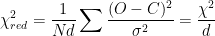
The need to do this stems from the fact that a quantitative analysis of data must be undertaken to seriously distinguish between two models whose goodness of fit to the data may not be as easily discriminated between in our “chi-by-eye” technique of just looking at them.

Large reduced chi-squared values indicate a poor model fit, and a value of 1 is typically sought but can be extremely difficult or impossible to achieve due to instrumental or intrinsic noise that are out of one’s ability to control. Values of the reduced chi squared that are less than 1 are typically a sign that you are “over-fitting” the model to the data. This can result from trying too hard to fit the model to noise, or overestimating the variance.

HD192263 RV Residuals

Above are the residuals to the HD 192263 dataset. This is keeping the x-axis (the time of the measurement) and plotting the O-C on the y-axis, instead of the radial velocity value for that data point. In this example, there is a trend in the data that has been modelled out which could potentially be due to a second orbiting companion that is far enough away that only a very small section of its orbit has been observed.

Other than the trend, there is no apparent structure in the residuals, and so there is no reason to suspect the existence of additional orbiting bodies.

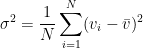
One can calculate the standard deviation, or variance, of the residuals to get a measure of how scattered the residuals are. This is typically represented with or written as ‘rms’ in literature, and is an algebraically obvious transformation of one of the above equations,

The radial velocity jitter of a star scales with both its mass and chromospheric activity. A quiet M dwarf may have a jitter as low as 2 to 3 metres per second, whereas a sun-like star may have a jitter on the order of 3 – 5 metres per second. F-type stars have jitters close to 10 metres per second, and the jitter sky-rockets from there, where A-type stars are nearly unusable for using radial velocity to detect extrasolar planets. As of the time of this writing, no planets have ever been discovered around an A-type star through the use of the radial velocity method. So there is an amount of variance in the residuals we should expect to have given the star we’re studying. If the variance is much higher than expected for the star, then it could be evidence of either unusually high stellar chromospheric activity, or as-yet undetected planets with small amplitude signals.

The systems we have looked at thus far throughout this blog in the context of radial velocity have been systems whose radial velocity data graphs are dominated by a single periodicity. Indeed, our own solar system is like this, with Jupiter dominating the sun’s radial velocity profile. But not all planetary systems come so conveniently organised.

I leave you with an image of how daunting this can be and why we are all thankful that computers are here to help us: An image of the 2008 three-planet fit for HD 40307 (since discovered to have three more planets).

HD 40307 Three-Planet Fit

---

Update (15 Apr 2013): I have corrected a math error in the equation for variance and standard deviation. In both cases the term should have been squared.

Tagged: HD 192263, HD 40307, Iot Dra, radial velocity, statistics