Modelling the Transit Light Curve

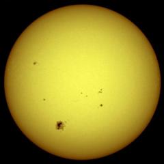
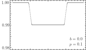
The Sun (Credit: NASA)

We looked at a simplistic understanding of planetary transits and transit light curves (here). In the interests of accuracy, it would be worth investigating a more formal understanding of the transit light curve. Specifically, this post will be aimed at actually modelling transit light curve while taking into account some more complicated dynamics such as limb darkening.

The actual shape of the transit light curve can be mathematically described by a function of the sky-projected centre-to-centre distance between the star and the planet, z, where z = 0 is understood to be the mid-transit of a centrally-crossing transit and the impact parameter, b is understood to be the minimum value of z throughout the transit, and the transit starts at about z ~ 1. More accurately, first and fourth contact start at , second and third contacts start at . Furthermore, let’s define p as the ratio of the radii of the planet and the star, .

Let us now define a function of the total fractional area of the star that is not obscured by the planet. Normally you might be inclined to feel that suffices, however it describes only the area ratio between second and third contacts, and is thus inadequate to describe the entire transit. We therefore will construct the amount of obscured stellar area as a piecewise function of p and z whose intervals describe different parts of the transit. It will be given as the ratio between the total area and the unobscured area subtracted away from the whole total area. Specifically, .

Where and . There’s a lot going on here but it isn’t too complicated to understand. The first case, , describes when the planet is completely off the stellar disc, before first contact hence there is no (zero) obscured area. The second case is the most complicated and describes the time between first and second (third and fourth) contacts. The third case is what we covered earlier, where the amount of obscured area is simply the square of the ratio of their radii, and therefore simply . The final case is only satisfied in the (unlikely) condition that the planet-to-star radius ratio > 1, and the entire area of the stellar disc is obscured.

Calculating z as a function of time may be done with knowledge of the impact parameter and use of Pythagorean theorem.

For a transiting planet with an impact parameter of zero and a radius ratio of (producing a 1% transit depth), the above model produces the following light curve plot.

Simulated Light Curve

Real light curves are actually curved, however, whereas this model is clearly much more “rigid” in shape. The reason for this is an effect known as limb darkening, where the outer layers of the star are not able to isometrically scatter light from underneath, causing less light from the limb of the star to reach the observer than from the centre of the stellar disc. For this reason, stars generally appear dimmer at their limbs and brighter in their centres. The magnitude of this difference will depend on a number of factors intrinsic to each star.

Proper handling of limb darkening will be required to obtain high-fidelity fits to high-accuracy data. A particularly popular and effective model for limb darkening was presented by Claret (2000). We can consider a four-parameter limb-darkening law describing the relative brightness of a point on the star expressed as a function of the angle between the observer, the centre of the star, and a line between the stellar centre and the given point on the star.

Where is given as , and each value of c is called a “limb darkening coefficient.” In the case of the centre of the stellar disc, . Each star will have a unique set of limb darkening coefficients, and they will change depending on what wavelength the transit is being observed in (due to how the properties of the stellar photosphere’s light scattering varies with wavelength). One could choose to have as many limb darkening parameters (and thus coefficients) as desired, but a high number is rarely required to adequately fit transit light curve data.

Limb darkening must be taken into account to get accurate measurements of radius ratios of transiting objects, and thus planetary radii. Because limb darkening will concentrate the brightness of the star into the centre of the disk, a planet that would cause a 1% transit depth in a uniformly bright star would cause a deeper transit depth in a central transit around limb-darkened star, and a shallower transit depth in a grazing transit around a limb-darkened star. Proper care in modelling the limb-darkening behaviour of the star is therefore required to ensure good measurement of the planetary radius.

We see therefore that the brightness difference is not a pure function of the ratio of the stellar and planetary radii. 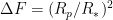is only an approximation, and only correct for the unrealistic case of a uniformly bright stellar disc.

So what can we do to get a more comprehensive representation of a light curve? Let’s modify the equation for we’re familiar with and consider brightnesses instead of just purely area ratios. Let’s take our limb-darkening equation as the radius of the star and determine the area, since it describes the brightness of the star from centre to limb. With this equation as the stellar “radius,” we use some simple calculus to expand it to the “brightness area” of the circle that is the stellar disc. This calculates the total brightness of the star while taking into consideration the changing brightness behaviour from centre to limb. The actual transit depth of a planet at any given distance to the centre of the star (represented as z again) is simply the ratio of the total stellar brightness in the area of the star under the planet to the total brightness of the stellar disc. Therefore, we draft a new function based off our original understanding of , while taking into effect the above model for how much of the star’s area is covered at any given time in the transit, as well as bringing in our limb-darkening model to describe the brightness distribution of the stellar disc:

And it makes quite a difference, too. By incorporating limb darkening coefficients, we’re able to much more accurately simulate the transit of a planet across a limb-darkened star. The diagram below shows the same planet (with p = 0.1) transiting stars of different limb-darkening parameters. The shape and modification to the transit depth is readily apparent.

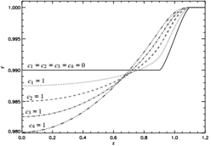
Effects of Limb-Darkening coefficients

Great Mysteries Revealed

Giant squid finally caught on video

It was recently announced that Japanese scientists have managed to finally capture video footage of a giant squid. We’ve known for some time that they exist, but until now, they have never been seen like this in their native environment.

Previously discussed detection methods for extrasolar planets leave much to be desired. Doppler spectroscopy tells you only a minimum mass for the planet and its orbital period. Transit photometry tells you the size and orbital period of the planet, and is typically not capable of confirming the detected object as a planet (since the mass is unknown, a brown dwarf or low-mass star could masquerade as a planet). Gravitational microlensing tells you the planet’s mass but only a projected distance from the star, and usually nothing about the orbit. Astrometry tells you the planet’s true mass and orbit in three dimensions, but otherwise permits you no more information about the planet than Doppler spectroscopy. Combining these techniques will allow one to tease out more information, but it’s still awfully indirect. We know the planets are out there, but it would be nice to actually see them.

The ultimate detection method of the future that will provide the most information is direct imaging. It’s very straightforward, all it involves is a large telescope with a decent imaging contrast ratio. It sounds easy but there are daunting challenges involved due to the proximity of planets to their stars and the brightness of their host stars.

The first directly imaged exoplanet

As of the time of this writing, only a couple dozen or so planets have been imaged with 8 – 10 metre class telescopes as well as HST. For the most part, they were all imaged in the infrared, they are all very massive as far as planets go, and they are all widely separated from their stars – typically hundreds of AU.

The greatest problem is that stars are very bright, and planets are comparatively very dim. In visible light, there’s a brightness contrast between the Sun and Jupiter of a factor of a billion, but depending on the wavelength and system age and planet mass, the brightness contrast can be as low as ten thousand. This problem is made worse by the diffraction of the starlight across the focal plane of the telescope produces a large amount of “noise,” with the star’s light spread out over a greater area of the image. A method of removing this excess light from a star is a requirement for directly imaging its planets.

One method of doing so is to use a coronograph. This is effectively an object in the telescope to block the light from the star, allowing one to see “around” the star. While you might therefore expect there to be dark “hole” in the image where the star is, the diffraction of light around the coronograph still produces a brighter, noisy area where the star would be. Imperfections in the coronograph will result in extra noise, and it is not clear that perfect coronographs are achievable. Since coronographs (even perfect ones) only attenuate the coherent part of the light’s wavefront (the shape of the waves of light). Imperfections in the wavefront (called aberrations) can leak through the coronograph to produce a residual noise in the form of a speckled halo around the star. Methods exist to correct this, such as wavefront correction with deformable mirrors or to calibrate images for speckles. It’s not perfect, but it certainly removes a lot of the excess starlight.

Four planets at HR 8799

Some caution is necessary when discovering planets through direct imaging. A supposed planet next to a star could turn out to be a background star. Monitoring of the planet candidate over some time will be needed to determine if it is bound to the star. Since stars and their associated planets move through space together, there is a certain motion in the sky that the planet and the star will follow if they are bound, whereas the two will have vastly divergent motions in the sky if they are not.

The advantages of directly imaging extrasolar planets is beyond having pictures – it permits direct spectroscopy of the planet’s light. Now while it is possible to gather information about the atmosphere of a transiting planet at a great distance from the star, the fraction of planets at large distances from their star that will transit are quite low. Direct imaging opens up access to all planets with a sufficient brightness and angular separation from the star.

I suspect in the future that this will be the most prevalent way of truly characterizing the planets in the solar neighborhood. Statistically speaking, few nearby Earths will transit, so we will require direct imaging to test their atmospheres for the presence of bio-markers that may be indicative of life.